I’ve often wondered why shared connection pools like PgBouncer are so popular compared to local, application-level pools. How much benefit do they really give, and why?
This post explores two main questions:
- For a single pool, how many open connections do we need to support a given workload?
- How does the number of open connections change as we increase the number of pools?
There are two ways of approaching this:
- Empirical: run experiments, either on a real database or using a simulation, and measure the connection usage under different configurations
- Analytical: build a mathematical model of the system, derive results using statistics
We’re going to do both! First run a simulation, then try to use statistics to explain the results, as well as giving a more intuitive explanation.
Simulation
The simulation models three application processes each making database queries. Each request acquires a connection, runs a single query, then releases the connection. Requests arrive according to a Poisson process, and query latency is drawn from a Gamma distribution.
Let’s compare two pool configurations:
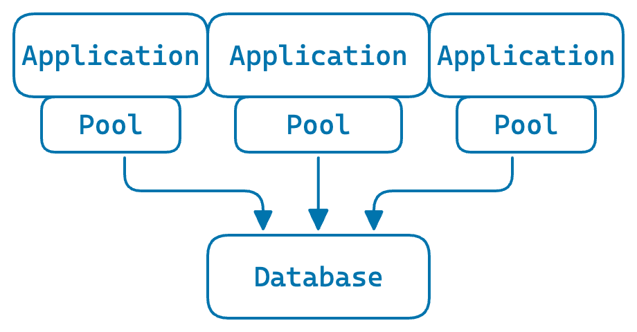
Local pools: each application process has its own pool
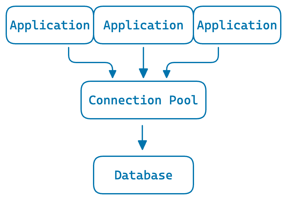
Shared pool: all processes share a single pool
The parameters:
- 200 requests per second total
- ~25ms average query latency – giving an average concurrency of around 5 (by Little’s Law: L = λW = 200 × 0.025)
- ~50ms average time to create a new connection
- 0.1% chance of destroying a connection after each use, to simulate connection churn
Assumptions: no maximum connection limit, no request queueing, and no network latency.
The code is available on GitHub.
A single pool
Let’s start with a single pool and the 200 RPS workload. With ~25ms average query latency, the average number of used connections – queries running at any moment – is around 5.
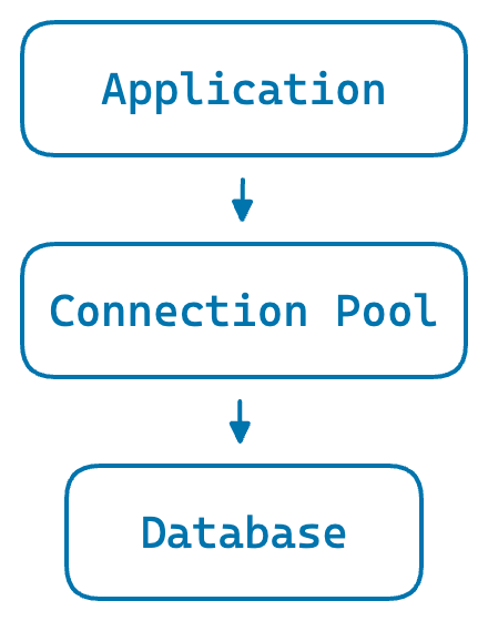
A single application process with its own pool
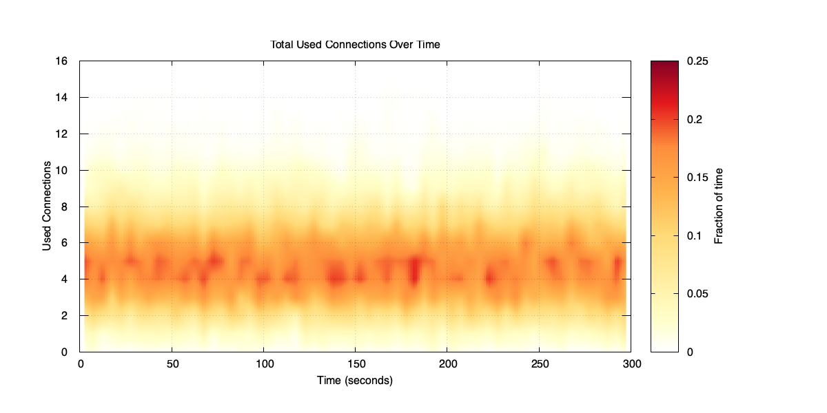
If we simulate 5 minutes of traffic, we can see how many connections the pool keeps open over time.
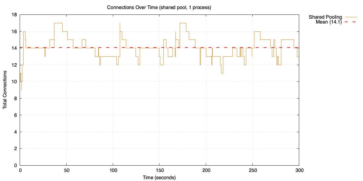
Open connections over time
The pool averages 14 open connections. That’s nearly three times the average used connections. Why?
It helps to look at the distribution of used connections.
Distribution of used connections over time
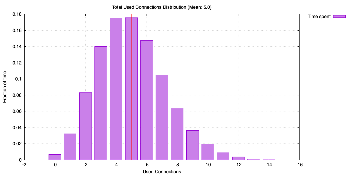
Histogram of used connections
Used connections can spike up to around 16, even though the average is 5. To understand why the pool size tracks the peaks rather than the average, consider two extremes.
Imagine a pool that creates a new connection for every request and destroys it immediately after. The number of open connections at any moment equals the used connections – averaging 5.
Now imagine a pool that never destroys connections. It keeps growing until it reaches the peak used connections, then stays there. Pool size approaches the maximum rather than the average.
Our pool sits in between. It keeps connections alive for reuse, but occasionally destroys one (0.1% of the time). So the pool size ends up much higher than the average used connections, but slightly lower than the maximum.
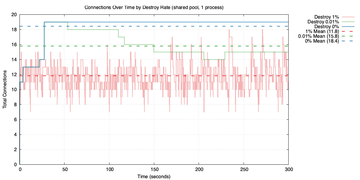
Pool size under different destroy rates
Higher churn means fewer idle connections kept around, so the pool stays smaller – but at the cost of creating connections more often.
Local vs shared
Let’s add two more application processes and see what happens.
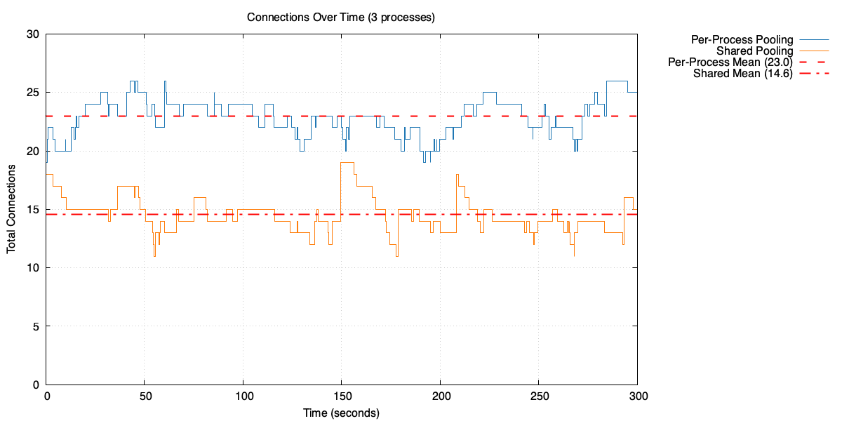
Open connections over time with three processes: per-process pooling vs shared pool
Each local pool needs fewer connections, but in total they need significantly more than the shared pool. In this case, the three local pools average around 23 open connections in total, compared to 14 for the shared pool.
Why though? Each local pool handles one third of the traffic, so the average used connections per pool drops to around 1.7 (average of 5 connections, divided by 3 processes). But each pool still has to handle its own peaks independently. Let’s look at the used connection distribution for a single process in the three-process case.
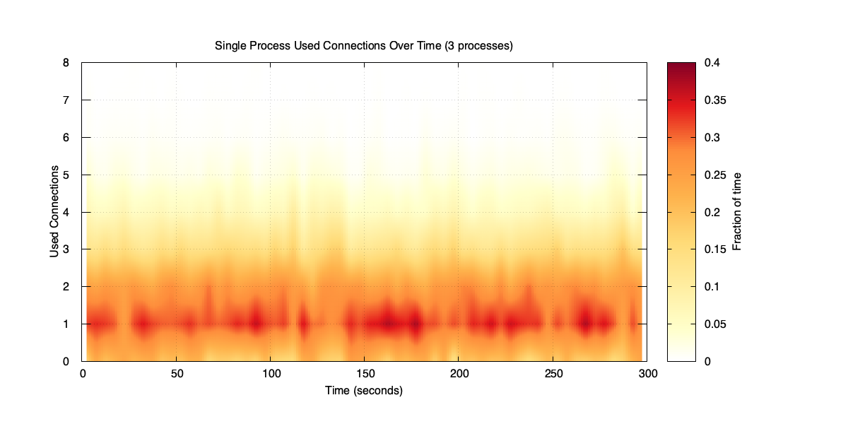
Used connections for a single process (three-process case)
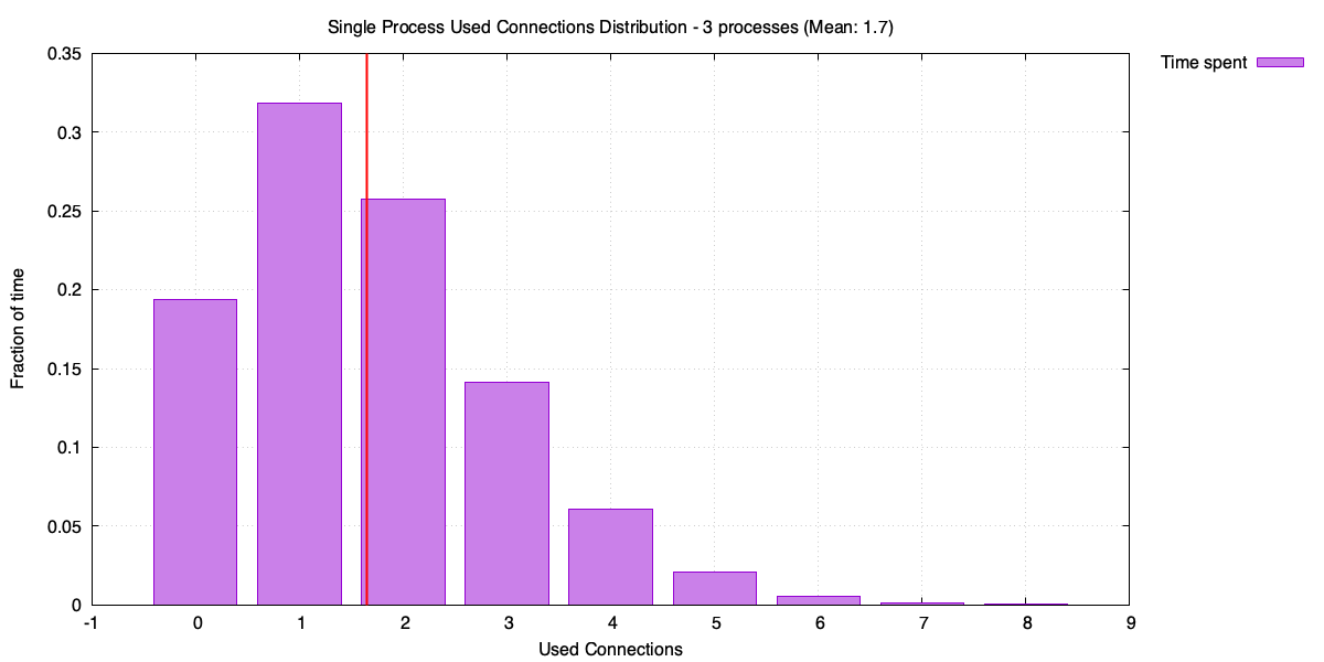
Distribution of used connections for a single process (three-process case)
It might not be obvious, but the distribution in this case is more spread out relative to its mean. Lower average traffic means more variability – the process spends a lot of time with zero or one used connection, but occasionally spikes. Each local pool has to be sized for those spikes, and with three pools doing the same thing independently, the total connection count adds up.
The shared pool, on the other hand, sees the combined traffic from all three processes. Individual spikes tend to average out, so the combined distribution is tighter relative to its mean.
Another way of thinking about it: each application process can use connections created by other processes’ requests, so they’re less likely to need a new connection. This results in fewer connections overall.
This is a property of the Poisson distribution. For a Poisson with arrival rate λ, the mean μ = λ and the standard deviation σ = √λ. As λ increases, σ also increases – but more slowly. The ratio σ/μ (standard deviation relative to the mean) gets smaller, meaning higher-traffic processes have proportionally less variability.
As λ increases, σ grows more slowly than the mean (μ)
The shared pool sees the combined traffic from all processes, so it effectively operates at a higher λ. Its distribution is tighter relative to its mean – it doesn’t need to keep as many spare connections around to cover rare spikes.
We can see this directly in the example below. Three independent Poisson distributions combine into a single Poisson with three times the mean. But the peak of the combined distribution is less than the sum of the three individual peaks.
Three Poisson(5) distributions combine into Poisson(15)
The difference between the sum of individual peaks and the combined peak – shown as 2.8 in the diagram above – is the saving from using a shared pool. Admittedly I’ve simplified the maths a bit by using one standard deviation above the mean as a proxy for the peak, but the principle holds.
The effect becomes even more pronounced with 10 processes.
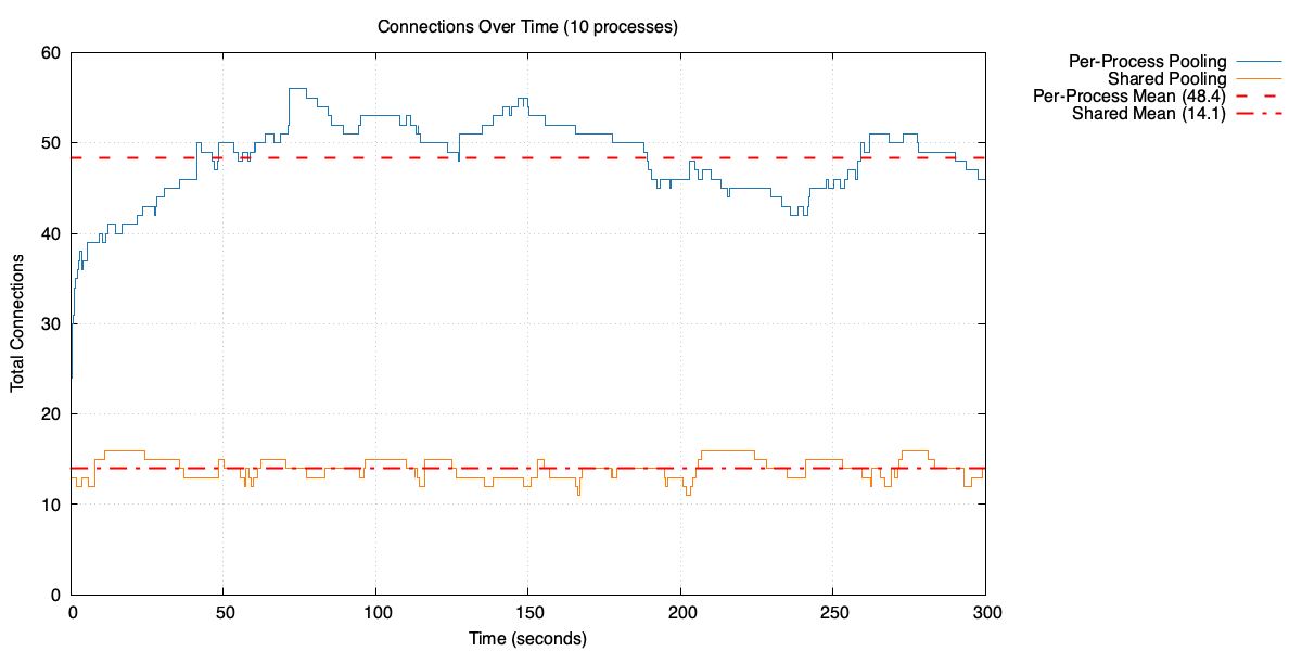
Open connections over time with 10 processes: per-process pooling vs shared pool
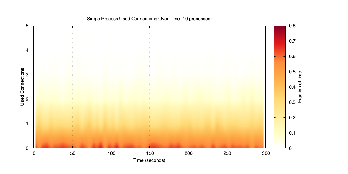
Used connections for a single process (10-process case)
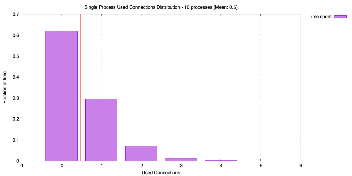
Distribution of used connections for a single process (10-process case)
Each process is now handling 20 RPS, averaging less than one used connection. The distribution is almost entirely zeros and ones, with rare spikes. The pools in total now need around 48 open connections to cover those spikes – up from 23 with three processes. Compare that with the shared pool sitting at around 14 open connections.
Practical implications
The simulation might be a simplification, but the principle applies to real systems. The more application processes you have, the more a shared pool helps. With a small number of processes the saving is modest, but with tens or hundreds it becomes significant.
A shared pool also helps during restarts and scale-out events. When a process restarts or a new replica comes up, it doesn’t need to spend time creating fresh connections – it can immediately borrow existing connections from the pool. This is especially valuable when connections are expensive to establish, as they often are with TLS and authentication overhead. For a concrete example, PostgreSQL’s SCRAM-SHA-256 authentication can add significant latency to connection establishment.
One big cost of a shared pool is the operational overhead of running another system. There’s also the extra network hop – queries go through e.g. PgBouncer rather than directly to the database. Whether that’s worth it depends on your setup, but for most applications with more than a handful of processes, the connection savings are substantial.